The CVA Python Package

The Python package cva allows you to use the design of experiments, automatic machine learning and optimization capabilities of ClearVu Analytics within Python. Before starting with machine learning you can easily set up design of experiments. For automatic machine learning this includes fitting, comparing, using, loading, saving and exporting models. In order to optimize, you can define objective and restrictions and can take advantage of the state-of-the-art optimizer.

The possibility of solution space optimization was introduced with ClearVu Solution Spaces. The idea is to find a box as big as possible within the design space, where all possible designs in the new box fulfill all given constraints. Thus, this is an optimization task (maximize the volume of the box with the constraint all designs in the box are valid.

Methods

Design of experiments

Design of experiments allow you a structured approach on generating new data. This can range from a simple Monte Carlo sampling to a Latin-Hyper-Cube sampling to an adaptive approach considering the quality of a model.

Automatic machine learning

Automatic machine learning includes the training of nonlinear models like neural networks, random forest and others and the optimization of the hyperparameter of the training algorithm. Afterward the different modeling approaches are compared and the best model can be selected. The optimization of the hyperparameters uses cross-validation with the aim to minimize the mean error on the validation part.

Evolutionary optimization

The general idea of evolutionary optimization is to mimic the cycle of generations in natural evolution. In evolutionary optimization a candidate solution is called ‘individual’. From an existing set of possible solutions, called parents, a larger set of individuals is created, using some implementation dependent algorithm. From this set of offsprings the best solutions are selected to be the parents for the next generation. This is repeated either for a number of generations or until a sufficient quality has been reached.

while i <= maxGeneration:
        # Create offsprings from parents.
        offsprings = self.next_offsprings(parents)
        # Adds fitness (quality) values to individuals.
        self.evaluate(offsprings)
        # Select parents for the next generation.
        parents = self.select(offsprings)
        i += 1

Solution space optimization

First, before diving into solutions spaces, you define the labels “good”/”bad” for designs (sample). A design is evaluated by one or more characteristics (e.g. quality, price, …) where for each characteristics exists a critical value. Thus, a good design fulfills all characteristics requirements where a bad design has one or more characteristics value beyond their critical value.

A solution space is a sub-space of a design space with the property of all designs within the sub-space being good. The optimization task is now to find a solutions space which is a big as possible. To check whether a sub-space is a valid solution space, a certain number of designs is evaluated in the sub-space.

Getting started

Design of experiments

First, you need to instantiate a manager to connect to the CVA core.

from cva import Base

manager = Base.Manager()

Then, create a design of experiment by

doe = manager.create_design_of_experiments()

A design of experiments needs at least a set of variables with limits (in case of real valued variables) and the method to use to generate the samples. The default is the Latin-Hyper-Cube method. Optional restriction functions can be added. For space-filling design an existing sample can be set. An adaptive strategy can be used in order generate samples with aim to improve a model. Hence, the model can also be added to the design of experiments.

Adding variables

For this example you add two real valued variables with a lower bound of -4.0 and an upper bound of 4.0.

doe.add_variable('x1', -4.0, 4.0)
doe.add_variable('x2', -4.0, 4.0)

you can change parameters by

doe.get_parameters()['NumExperiments'].set_value(100)

This sets the size of sample to 100. To get an overview of the current parameters use

print(doe.get_parameters())

Generating the samples

to actually generate the samples start

df = doe.create_design_of_experiments()

The new samples are returned as a pandas.DataFrame. You can also get the samples later with

df = doe.get_doe()

Automatic machine learning

First, you need to instantiate a manager to connect to the CVA core.

from cva import Base

manager = Base.Manager()

Preparing models

The manager object can be used to create or import models. To create a model use

model = manager.create_model('neural_network')

The list of available model types can be get with available_model_types(). The model object contains information on how the model will be trained. Therefore, a set of model independent task parameter and a set of model specific parameter can be set. The default values can be shown using

model.get_fit_task().get_task_parameters()
model.get_fit_task().get_model_parameters()

Each parameter is of type cva.Structures.CvaParameter. To change for example the flag for calculating the variable importance, use:

model.get_fit_task().get_task_parameters()['DoCalcVariableImportance'].set_value(False)

Cross-validation and optimization are on by default.

Fitting models

In order to fit a model you need a data frame with the data, the names of the input variables (column names) and the name of the output variable (column name). This package includes some sample data (cva.Examples). The next example uses data generated with the Rosenbrock function.

from cva import Examples

example = Examples.data_rosenbrock()
input_variable_names = example['input_variable_names']
output_variable_name = example['output_variable_names'][0]

Now you can fit the model with

model.fit(example['df'], input_variable_names, output_variable_name)

The fit function returns True on success and False, if it is impossible to fit the model. Detailed information can be obtained using the function

info = model.get_fit_info()

which returns a cva.Structures.CvaModelInfo object. It contains information on quality characteristics, input variable importance, input variable sensitivity and validation prediction values. For more information refer to cva.Structures.CvaModelInfo.

There are some additional shortcuts to access the information directly.

# Quality values
df_quality = model.get_qualities()

# Variable importance
df_importance = model.get_variable_importance()

# Variable sensitivity
df_sensitivity = model.get_variable_sensitivity()

# Cross-validation values
df_scatter = model.get_validation_data_frame()

# For classification
df_confusion = model.get_confusion_matrix()

Using models

In general, you would like to use the models to predict the outcome of new data. This is done with the fit function.

y, c = model.predict(df)

Note that not only the predictions y are returned, but also a confidence value for each prediction c. The confidence value is between zero and one. One means that the possibility of the prediction being right is very high while a low confidence value reduces this possibility. The calculation of the confidence uses the next neighbors with in the learning data of the new data point and the variances of the output values. The distances are used weight the influence of the neighbors. There are some parameters which can be used to adjust the conficende calculation.

• You can limit the maximal number of neighbors (-1 would use all learning data).

• You can define a maximal reach of a data point. Thus, only neighbors which are within a certain distance are used for the calculation. All values are normed to the interval [0, 1]. The maximal reach is defined by a fraction of the diagonal of the design space (\(\sqrt{n}\), \(n\) = number of dimensions).

The default is just restricting the reach by 20% of the diagonal. You can change the values after a model fit with

# Limit the number of neighbors to 20
model.set_model_parameter('ConfidenceK', 20)

# Allow further reach (50% of the diagonal)
model.set_model_parameter('ConfidenceThreshold', .5)

You can switch off confidence calculation with the optional parameter confidence set to False.

y, c = model.predict(df, confidence = False)

In this case, c is a list of NaNs.

Comparing models

One great advantage of CVA is the possibility to compare the resulting different models for one task and rank them and pick automatically the best one for the given task. Before starting to compare just fit some different models for one task.

from cva import Examples

example = Examples.data_rosenbrock()
input_variable_names = example['input_variable_names']
output_variable_name = example['output_variable_names'][0]
models = [manager.create_model(model_type) for model_type in manager.available_model_types()]
fit_task = models[manager.available_model_types().index('random_forest')].get_fit_task()
fit_task.get_model_parameters()['mtry'].set_value(2)
[model.fit(example['df'], input_variable_names, output_variable_name) for model in models]

Note, that you need to adapt the mtry parameter for a random forest if you have only two variables. Now you have ten different models for the same task. To compare the models use

comp = manager.compare_models(models)

cva.Base.Manager.compare_models() returns a list of comparisons. The elements are grouped by input variables sets and output variable names. In this case there is just one entry. To get the best model use

winner = comp[0].get_winner()

To get the ranking use

wins = comp[0].get_wins()

A sorted list of tuples of the model and how many times it won against other models is returned. To get a complete overview use

matrix = comp[0].get_matrix()

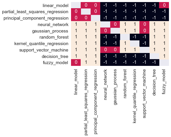
A matrix with pairwise comparison is returned. A -1 means row lost against column, 0 no significant difference, 1 row won against column (see also cva.Structures.CvaModelCompare.get_matrix()). You can visualize this for example using seaborn.

import seaborn as sn

sn.set(font_scale=1.4)
sn.heatmap(comp[0].get_matrix(), annot=True, annot_kws={"size": 16})

This results in the following chart:

Managing models

You can export the model using the function cva.Models.Model.export(), which writes an xml file which can be used with other CVA tools. Alternatively, you can use pickle to save the model. To import an xml file use cva.Base.Manager.import_model(). To reload from a pickle you can either use the function cva.Base.Manager.load_model() or use unpickle and then connect the model with manager via cva.Models.Model.connect(). New data can be predicted with the model function cva.Models.Model.predict(). The predict function returns a tuple of the predicted value and a confidence value. The confidence value is between one and zero, with one being the highest confidence.

Ensemble models

Ensemble models are a type of models that uses several existing models and predicts data with these models in several ways. The possible predict types are

• mean_predict: calculates the mean of the predictions of all models

• mean_weighted_predict: calculates the mean of the predictions of all models multiplied by their confidence

• best_predict: returns the best predictions of each value by the confidence

With the cva.Base.Manager.create_ensemble_model() method you can make a new ensemble model. You can also set the predict mode here or later, ‘mean_predict’ is the default.

ensemble_model = manager.create_ensemble_model(models, manager, predict_mode='mean_predict')

After you created the ensemble model, You can set the predict mode.

ensemble_model.set_predict_mode('mean_weighted_predict')

Now you can use the predict method of the ensemble model like any other model, too.

y,c = ensemble_model.predict(df)

You can change the predict mode at any time, so you could do the following:

ensemble_model.set_predict_mode('mean_predict')
y1,c1 = ensemble_model.predict(df)
ensemble_model.set_predict_mode('mean_weighted_predict')
y2,c2 = ensemble_model.predict(df)
ensemble_model.set_predict_mode('best_predict')
y3,c3 = ensemble_model.predict(df)

User defined models

In addition to the provided modeling algorithms, you can use or implement your own modeling algorithms and integrate them into the cva framework. All you need to do is to implement a wrapper class providing certain functions. To work, the flask package is required.

The following example wraps the regression tree from sklearn. You can use the template class cva.Models.UserModelInterface as a basis for the implementation of a new wrapper.

class UserModelInterface:
        '''
        Template class for building a user model. The user model class can be derived from this class. The actual implementation
        of the user algorithm must be given as a reference to the constructor and must work with pickle for storing/loading.

        .. hint:: A user model is created using the function :py:meth:`cva.Base.Manager.create_user_model` with an object implementing the function of this interface.

        .. code-block:: python
                :linenos:

                y, c = model.predict(df, confidence = False)
        '''

        def __init__(self, model) -> None:
                self.model = model

        def get_parameter_list(self, input_cnt) -> list:
                ''' This function should return the list of parameters / hyper-parameters which can be configured or optimized.

                Args:
                        input_cnt: In order to properly initialize the parameters, the number of input variables is provided.

                Returns:
                        A list of parameters of type :py:class:`cva.Base.Structures.CvaModelParameter`.
                '''
                return []

        def set_parameter_values(self, parameter_values) -> None:
                ''' This function changes the current parameter values.

                Args:
                        parameter_values: A dictionary of name value pairs for the parameters to be changed.
                '''
                pass

        def fit(self, df, input_variable_names, output_variable_name) -> None:
                ''' The fit function should provide the actual training algorithm for the user model. The resulting model should be stored in self.model.

                Args:
                        df: Learn data as data frame.
                        input_variable_names: List of input variable names.
                        output_variable_name: Name of the output variable.
                '''
                pass

        def predict(self, df, input_variable_names, output_variable_name):
                ''' Predict values using new data.

                Args:
                        df: Data frame to predict.

                Returns:
                        A pandas.DataFrame containing one column "output_variable_name" with predictions.
                '''
                pass

The model object passed to the constructor holds all information to store and load a model. An implementation of a wrapper for the regression could look like

import pandas as pd
from cva.Models import UserModelInterface
from cva.Structures import CvaModelParameter
from sklearn import tree

class SklearnDecisionTreeRegressor(UserModelInterface):

        def __init__(self):
                super().__init__(tree.DecisionTreeRegressor())

        def get_parameter_list(self, input_cnt) -> list:
                param_list = [
                        CvaModelParameter(name='criterion',
                                value='poisson',
                                value_type='enum',
                                description='The function to measure the quality of a split.',
                                enums=['squared_error', 'friedman_mse', 'absolute_error', 'poisson'],
                                is_optimizable=True),
                        CvaModelParameter(name='max_depth',
                                value=min(input_cnt, 1),
                                value_type='integer',
                                description='Maximal depth of the tree.',
                                is_optimizable=True,
                                opt_min=1,
                                opt_max=input_cnt),
                        CvaModelParameter(name='min_samples_split',
                                value=20,
                                value_type='integer',
                                description='Minimum needed number of samples in order to split.',
                                is_optimizable=True,
                                opt_min=2,
                                opt_max=100)]
                for param in param_list:
                        self.model.set_params(**{param.get_name(): param.get_value()})
                return param_list

        def set_parameter_values(self, parameter_values):
                for name, value in parameter_values.items():
                        self.model.set_params(**{name: value['value']})

        def predict(self, df, input_variable_names, output_variable_name):
                X = df.loc[:, input_variable_names].to_numpy()
                return pd.DataFrame(index=range(len(df)), data={output_variable_name: self.model.predict(X)})

        def fit(self, df, input_variable_names, output_variable_name):
                X = df.loc[:, input_variable_names].to_numpy()
                y = df[output_variable_name].to_numpy()
                self.model.fit(X, y)

In the constructor you instantiate the regression tree. The :py:meth:get_parameter_list returns the list of parameter used for training. Note, that all parameters will be optimized while training. The new class can be used straight forward.

from cva import Base, Examples

example = Examples.data_rosenbrock(100)
input_variable_names = example['input_variable_names']
output_variable_name = example['output_variable_names'][0]
df = example['df']

manager = Base.Manager(with_flask=True)

model = manager.create_user_model(SklearnDecisionTreeRegressor())
model.fit(df, input_variable_names, output_variable_name)

The new model acts as any of the other models. Thus, confidence value calculation, hyperparameter optimization and cross-validation is included. The only thing not possible is the export to other ClearVu Analytice tools.

Optimization

First, you need to instantiate a manager to connect to the CVA core.

from cva import Base

manager = Base.Manager()

The manager object can be used to create or import optimizations. To create an optimization use

optimization = manager.create_optimization()

An optimization task needs to know what to optimize and which values to change in order to achieve that. You need to set at least one objective function, at least one input variable. Optional restriction functions can also be added.

Adding variables

For this example, You add three real valued variables with a lower bound of -100.0 and an upper bound of 100.0.

optimization.add_variable('x1', -100.0, 100.0)
optimization.add_variable('x2', -100.0, 100.0)
optimization.add_variable('x3', -100.0, 100.0)

Implementing an evaluation function

The aim of an optimization can be to reach one or more objectives and optionally fulfill a number of restrictions. You need to implement a function accepting a data frame and returning a data frame with objective and restriction values. Each iteration, the candidate solution spaces are sent as data frame to the evaluation function. The data frame contains a column for each input variable and as many rows as set by the parameter Lambda explained later. The function needs to return a data frame containing a column for each objective/restriction and the same number of rows. The names of the objective/restriction columns must match the names set in the optimization. The names of all objectives/restrictions need to be unique.

The package includes two examples of evaluation functions:

• cva.Examples.optimization_single_objective_evaluation(): A function using cva.Examples.function_sphere() and cva.Examples.function_restriction() to evaluate candidates. This function is used to demonstrate the case of a single objective with one restriction.

• cva.Examples.optimization_multi_objective_evaluation(): A function using cva.Examples.function_sphere() and cva.Examples.function_rosenbrock() to evaluate candidates. This function is used to demonstrate a multi-objective case with two objectives.

Adding objectives

The minimum information needed to set an objective function is a name. The same name must be used as the name of the column that will contain the values for this objective or restriction function in the evaluation function. These values are calculated by the evaluation function, which has to be implemented and set by you. First, you add an objective with cva.Optimizations.Optimization.add_objective():

# Announce an objective function called 'function_sphere'
optimization.add_objective('function_sphere', 'Minimize')

Adding restriction functions

The parameters of the cva.Optimizations.Optimization.add_restriction() function are name, operator, and value. Again, the name has to be the identifier for the data column which will contain the restriction values, calculated by the evaluation function. Operator must be one of ‘<’, ‘<=’, ‘>=’, ‘>’.

# Announce a restriction function called 'function_restriction'
optimization.add_restriction('function_restriction', '>', 5.0)

The example restriction function calculates the sum of x1 and x2. A candidate is valid if the value is greater than 5.0.

Setting the evaluation function - the actual optimization problem

A function pointer to objectives and restrictions functions can be set with:

from cva import Examples

optimization.set_evaluation_function(Examples.optimization_single_objective_evaluation)

The evaluation function has a simple interface and needs to be implemented by you. The function takes a data frame as input parameter. Each row in this data frame should contain values for all input variables. The data frame returned by this function has to contain the calculated objective and restriction values. The returned data frame may also contain the input values, which makes it easier to use the DataFrame.apply function.

Changing optimization parameters

Parameters of the optimization can be changed with the cva.Optimizations.Optimization.set_parameter() function. Most important parameter you may want to change are the number of generations, that will be generated, and the two size parameters ‘Mue’ and ‘Lambda’. ‘Mue’ is the size of the parent population, and ‘Lambda’ is the size of the offspring population. Please keep in mind, that the parameter values in this example have been tuned down for a very simple objective function and may be not sufficient for our task. An initial set of four individuals will be created. The two best individuals will be selected, and the optimization loop will be run ten times. In each iteration four new individuals will be created, and the two best individuals will be selected for the next step. This leads to total of 44 created and evaluated individuals (4 initial and 10*4 within the loop).

optimization.set_parameter('MaxGeneration', 10)
optimization.set_parameter('Mue', 2)
optimization.set_parameter('Lambda', 4)

Starting the optimization

After finishing the setup of the optimization it can be started with:

bests = optimization.start()

When the optimization finishes successfully, the optimal solutions are returned.

Optimization history

To get the complete history of the optimization run, you can use the cva.Optimizations.Optimization.get_history() function. The returns data frame contains all candidate solutions, including the associated objective and restriction function values. The ‘type’ column contains information about creation and selection of individuals. The ‘generation’ column contains the generation that the individual belongs to, which is the iteration counter i, as described above in the evolutionary optimization loop.

history = optimization.get_history()

	x1	x2	x3	function_sphere	function_restriction	generation
…	…	…	…	…	…	…
10	48.70	1.14	-25.99	4017.83	79.84	1
11	53.22	6.94	-39.40	4433.68	60.16	1
12	73.92	36.42	-44.27	8752.69	110.35	2
13	58.86	13.99	-63.97	7753.04	72.85	2
14	42.11	58.03	-57.63	8463.68	100.15	2
15	75.88	-9.28	11.42	5975.30	66.59	2
…	…	…	…	…	…	…

The optimization class allows you to optimize a single or multiple objective functions. The following chart shows the complete history of an optimization run in a box plot:

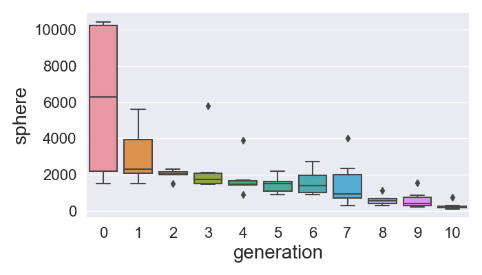
This plot has been created basically with the following lines:

import seaborn as sn

box = sn.boxplot(x = 'generation', y = 'function_sphere', data = history)

Multi-objective optimization

You can optimize multiple objective functions simultaneously. Just add another function name and calculate the according values in you evaluation function.

optimization.add_objective('function_rosenbrock')

It is also possible to remove objects from the optimization. To remove the restriction function you can use:

optimization.remove_restriction('function_restriction')

Now you set the new evaluation function

optimization.set_evaluation_function(Examples.optimization_multi_objective_evaluation)

Now, the optimization can be started again. Using the cva.Optimizations.Optimization.start() method triggers a complete optimization run from initialization to returning results. Previously generated results will be replaced.

result = optimization.start()

The sphere function has its minimum at

\[f(x_{1},...,x_{n}) = f(0,...,0) = 0\]

The Rosenbrock-function has its minimum at

\[f(x_{1},...,x_{n}) = f(1,...,1) = 0 \quad | \quad n \geq 2\]

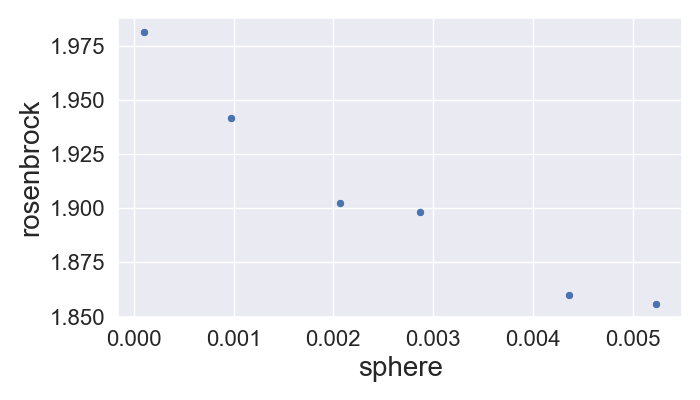
This means that it is impossible to find a single perfect solution. And in this case the optimization will find a set of ‘Pareto-equivalent’ solutions (named after Vilfredo Pareto). Pareto-optimality describes the situation where no objective function value can be better off without any loss of quality in at least one other objective.

Using

sn.scatterplot(x = 'function_sphere', y = 'function_rosenbrock', data = result)

gives the following chart:

Continue optimization

In case insufficient optimization results, you can continue the optimization by calling the cva.Optimizations.Optimization.continue_run() method. It only parameter is the number of additional generations to perform.

optimization.continue_run(100)
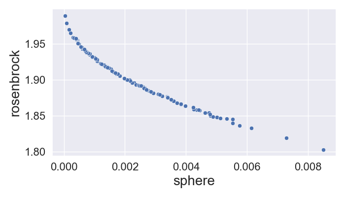
result = optimization.get_result()

Which leads to a larger set of Pareto equivalent solutions:

Managing optimizations

You can use pickle to save the optimization. To reload from a pickle you can either use the function cva.Base.Manager.load_optimization() or use unpickle and then connect the model with the manager via cva.Optimizations.Optimization.connect().

Solution space optimization

First, you need to instantiate a manager to connect to the CVA core.

from cva import Base

manager = Base.Manager()

The manager object can be used to create or import solution space optimizations. To create an optimization use

space_opt = manager.create_solution_space_optimizer()

In order to define a solution space optimization task, you need to define the input space and the outputs (deciders for good/bad designs). The input space is defined by a set of input variables either real-valued or class variables. Additionally, you need to define the range for each variable (lower/upper bound for real-valued variables, a set of class labels for class variables).

Defining the input space

For this example you add two real-valued variables with a lower bound of -4.0 and an upper bound of 4.0 and a class variable with three classes.

space_opt.add_input('x1', -4., 4.)
space_opt.add_input('x2', -4., 4.)
space_opt.add_input('x_class', labels = ['green', 'yellow', 'red'])

Setting the output variables

Next, you define one output variable with a critical upper value of 500 meaning any design with a value higher than 500 is considered bad.

space_opt.add_output('y', upper_crit=500)

Implementing an evaluation function and setting it

Similar to standard optimization described above, you need an evaluation function which calculates the output values for a set of designs. Therefore, you need to implement a function accepting a data frame and returning a data frame with output variable values. Each iteration, the candidate solution spaces are evaluated by creating a set of samples for each candidate and these are sent to the evaluation function to obtain the output values. The data frame containing the samples has a column for each input variable. The function needs to return a data frame containing a column for each output variable and the same number of rows as the input data frame. The names of the output variable columns must match the names set in the optimization. The names of all output variables need to be unique.

In this example you use a modified Rosenbrock function.

from cva import Examples

def evaluation_function(df):
        y = []
        for row in range(len(df)):
                y_rosenbrock = Examples.function_rosenbrock(df.iloc[row,0:2])
                if df.iloc[row, 2 ] == 'yellow':
                        y_rosenbrock *= y_rosenbrock
                if df.iloc[row, 2 ] == 'red':
                        y_rosenbrock *= y_rosenbrock
                y += [y_rosenbrock]
        return pandas.DataFrame(data={'y': y})

An evaluation function is connected to an optimization with:

space_opt.set_evaluation_function(evaluation_function)

Final solution space quality

The aim of a solution space optimization is to maximize a box where all designs are good designs. To avoid that an edge is preffered over others because of a different scale about measure for the quality of a solution space should be based on normalized edges. A straight forward measure would be the volume of the solution space. But, this measure can encounter numerical issues with high input dimensions. An alternative can be the sum of the edges which is measure selected by default.

To add flexibility, the box evaluation function can be changed with:

space_opt.set_box_evaluation_function(box_evaluation_function)

A box evaluation function takes as box (dictionary of name -> [min, max] or name -> [class_name_1, class_name_2, …]) and returns the quality as a scalar value (higher -> better). There are some predifined functions available:

cva.Optimizations.SolutionSpaceOptimization.box_norm_volume()

def box_norm_volume(self, box):
        widths = [interval[1]-interval[0] for variable_name, interval in box.items()]
        return numpy.prod(widths)

cva.Optimizations.SolutionSpaceOptimization.box_norm_diagonal()

def box_norm_diagonal(self, box):
        widths = [interval[1]-interval[0] for variable_name, interval in box.items()]
        return numpy.sqrt(numpy.sum(numpy.square(widths)))

cva.Optimizations.SolutionSpaceOptimization.box_norm_edge_sum()

def box_norm_edge_sum(self, box):
        widths = [interval[1]-interval[0] for variable_name, interval in box.items()]
        return numpy.sum(widths)

cva.Optimizations.SolutionSpaceOptimization.box_norm_weighted_edge_sum()

def box_norm_weighted_edge_sum(self, box):
        widths = [interval[1]-interval[0] for variable_name, interval in box.items()]
        widths.sort()
        return numpy.sum(numpy.multiply(widths, [i for i in range(len(widths), 0, -1)]))

For example, you can change from edge sum to diagonal with:

space_opt.set_box_evaluation_function(space_opt.box_norm_diagonal)

Changing optimization parameters

Parameters of the optimization can be changed with the cva.Optimizations.SolutionSpaceOptimization.set_parameter() function. The most important parameter you may want to change are the number of generations, that will be generated, and the two size parameters ‘Mue’ and ‘Lambda’. ‘Mue’ is the size of the parent population, and ‘Lambda’ is the size of the offspring population. Please keep in mind, that the parameter values in this example have been tuned for a very simple objective function and may be not sufficient for our task. The parameter ‘TestSampleCount’ sets the number of samples for each candidate box used to evaluate a candidate. Thus, in total lambda * max_generations * test_sample_count sample designs will be evaluated during an optimization.

space_opt.set_parameter('Mue', 5)
space_opt.set_parameter('Lambda', 10)
space_opt.set_parameter('MaxGeneration', 100)
space_opt.set_parameter('TestSampleCount', 100)

Constraining the search space for real-valued input variables

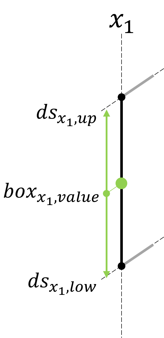
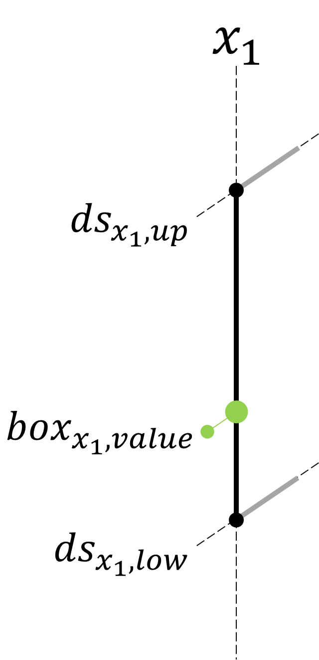
Usually, if looking at one variable (edge), the solution space optimizer tries to find an edge which is inside the design interval. For a variable \(x_1\) the design interval is given by the lower bound \(ds_{x_{1},low}\) and the upper bound \(ds_{x_{1},up}\). You can change the design interval with cva.Optimizations.SolutionSpaceOptimization.set_input_lower_bound() and cva.Optimizations.SolutionSpaceOptimization.set_input_upper_bound(). One of the bounds can be fixed with either cva.Optimizations.SolutionSpaceOptimization.set_input_is_lower_fixed() or cva.Optimizations.SolutionSpaceOptimization.set_input_is_upper_fixed(). If both are fixed, the input variable is not used in the optimization. The interval is still used as the sampling interval for this input variable.

Default setting for an input variable	Fix the lower bound of an input variable
space_opt.set_input_lower_bound('x1', 0.) space_opt.set_input_upper_bound('x1', 1.)	space_opt.set_input_is_lower_fixed('x1', True)

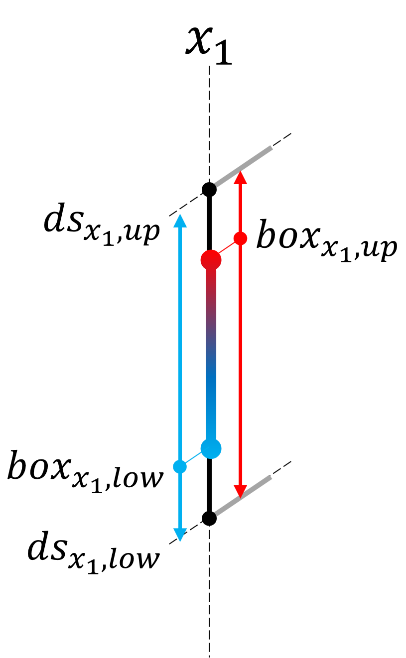
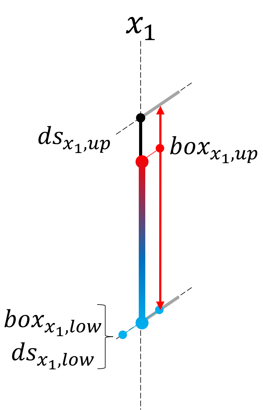
For the default both \(box_{x_{1},low}\) and \(box_{x_{1},up}\) of the final solution space box can be anywhere in the design interval except that \(box_{x_{1},up}\)> \(box_{x_{1},low}\). This default setting can be altered for each variable indivdually in order to constrain the solution, like fixing one bound.

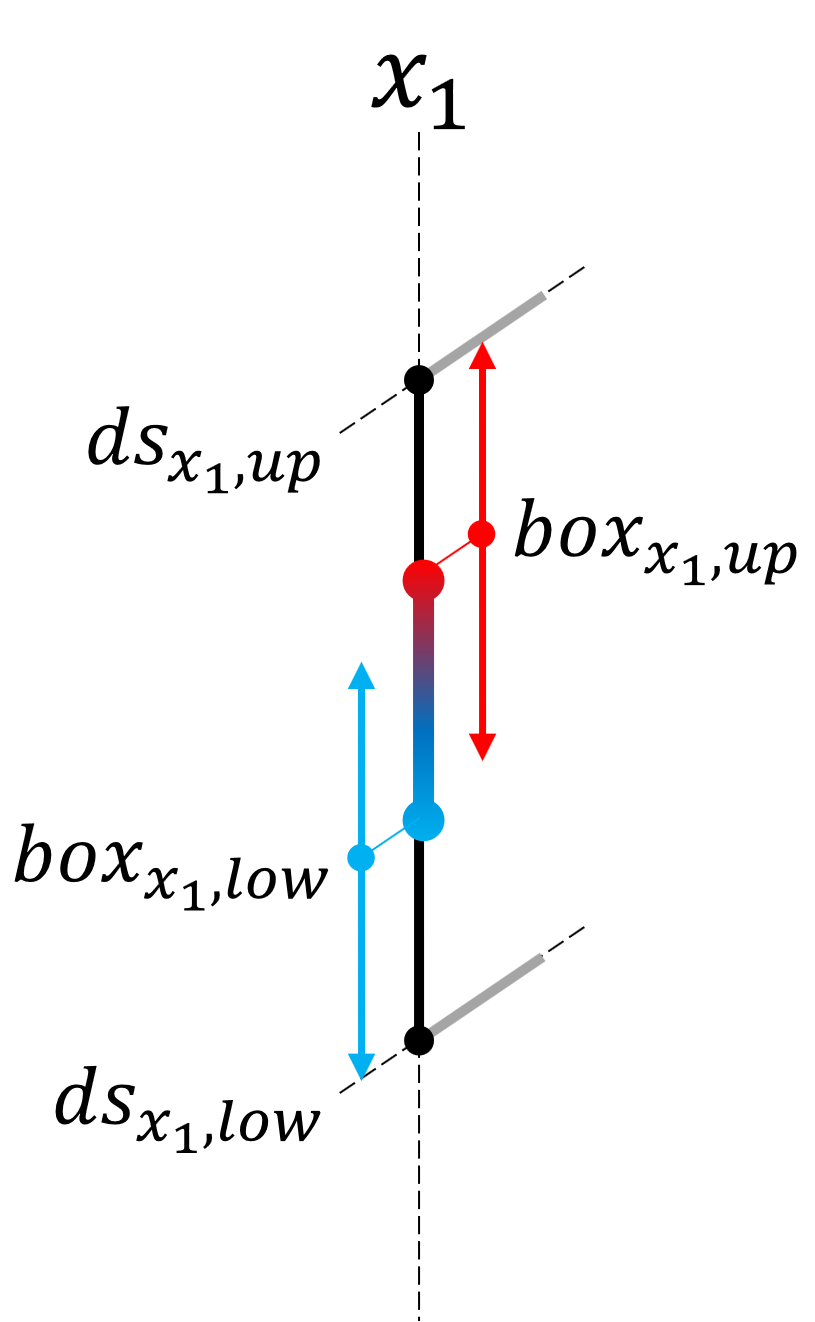
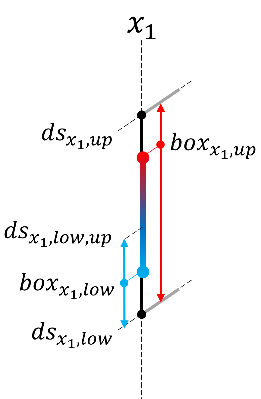
There are two additonal options to constrain an input variable. The width of the final interval can be fixed with cva.Optimizations.SolutionSpaceOptimization.set_input_is_width_fixed() and cva.Optimizations.SolutionSpaceOptimization.set_input_width(). The other option is to set additonal bounds for the lower and upper bound (cva.Optimizations.SolutionSpaceOptimization.set_input_lower_upper_bound() and cva.Optimizations.SolutionSpaceOptimization.set_input_upper_lower_bound()). In the example below the lower bound is constraint by a seperate upper bound which differs from the design interval upper bound.

Fix the width of an input interval	Additionally constrain the lower bound
space_opt.set_input_is_width_fixed('x1', True) space_opt.set_input_width('x1', .5)	space_opt.set_input_lower_upper_bound('x1', .4)

If a variable should have a certain value instead of allowing an interval you can use cva.Optimizations.SolutionSpaceOptimization.set_input_is_interval() and set interval to False. In addition the value can be fixed (cva.Optimizations.SolutionSpaceOptimization.set_input_is_value_fixed() and cva.Optimizations.SolutionSpaceOptimization.set_input_value()), thus this variable is not used in the optimization.

Single value instead of an interval	Fixed value for an input variable
space_opt.set_input_is_interval('x1', False)	space_opt.set_input_is_interval('x1', False) space_opt.set_input_is_value_fixed('x1', True) space_opt.set_input_value('x1', 0.3)

Constraining the search space for class input variables

By default, the result of an edge represented by class variable is a subset of the labels defined in the design space. You can fix the edge to the defined classes with cva.Optimizations.SolutionSpaceOptimization.set_input_is_class_names_fixed(). If only one class label should be selected as an edge, cva.Optimizations.SolutionSpaceOptimization.set_input_is_interval() must be set to False. If in addition the single label edge is also fixed use cva.Optimizations.SolutionSpaceOptimization.set_input_is_value_fixed() and set the fixed label with cva.Optimizations.SolutionSpaceOptimization.set_input_value().

Starting the optimization

After finishing the setup of the solution space optimization it can be started with:

results, qualities = space_opt.optimize()

When the optimization finishes successfully, the optimal solution spaces and their qualities are returned.

The following chart shows how the solution space optimizer works:

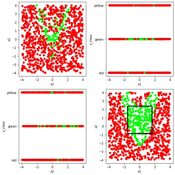
If you create random samples in the design space and assign the colors green=good / red=bad and plot them like in the upper left chart, you see the difficulty to define a box which gives only good samples, as the result also depends on the x_class. After the optimization you get a plot like the one in the lower right corner if you sample the dependent variables (in this case x_class) within the bounds of the optimal solution space.

More options to control the optimization

It is possible to further restrict the optimization in the design space. This includes fixing bounds of input variables, using single value instead of an interval/class set to setting a fixed width for real-valued input variables. Also, you can provide initial boxes instead of letting the optimizer generate random start boxes.

Managing solution space optimizations

You can use pickle to save the optimization. To reload from a pickle you can either use the function cva.Base.Manager.load_solution_space_optimizer() or use unpickle and then connect the model with the manager via cva.Optimizations.SolutionSpaceOptimization.connect().